
As the scientific community continues to generate ever-increasing volumes of data, obtained through experiments or numerical simulations, machine learning has emerged as an increasingly popular tool among researchers across different scientific domains.
Quantemol aims to leverage available data sources, including the Quantemol Database (www.quantemolDB.com) alongside other scientific databases and research publications, to craft data-driven solutions for addressing challenges within the plasma modelling community.
We have previously developed a machine learning–based algorithm for fast estimation of unknown heavy particle collisions rate coefficients using commonly available chemical species data [ref 1]. Apart from that, we have designed algorithms to predict missing species data, including standard enthalpy of formation and dipole moment. Our current focus revolves around developing a machine learning model to estimate mass spectrometry data for inferring electron impact ionisation fragmentation patterns. These branching ratios are critical for plasma chemistry modelling and predicting important species concentrations in plasma discharge.
Here we delve into the key steps of our machine learning journey throughout a project, from data collection and preparation to model selection and training, offering insights into the crucial role of data and the potential of machine learning in designing solutions for problems relevant to plasma modelling.
Step 1 : Data gathering
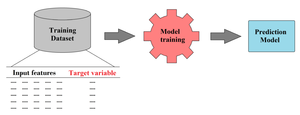
Every machine learning project starts with the process of gathering data. Besides collecting the outputs (or targets) that we want to predict, we need to gather as much as possible data that can be used to create model inputs (or features) so the final dataset can enable the model to learn and make accurate predictions based on the available data patterns and relationships.
On one hand building a robust machine learning model requires a significant volume of data, yet the quality of data is equally important. To ensure our model can identify the right patterns, we collect data only from reliable sources such as online scientific databases (including Quantemol Database) and individual scientific publications.
Step 2: Data preparation
After collecting all the relevant data, we need to prepare it to be suitable for model training.
Our data preparation pipeline typically involves the removal of inconsistent and duplicate values, handling outliers and missing data, target variable transformation, feature engineering and scaling.
Most machine learning algorithms cannot handle missing data. Ideally we should aim to collect all the necessary data for all the instances, but in practice, our data set will always have a portion of missing values. Restricting the dataset to include only instances with complete values would significantly reduce the dataset’s size. To avoid this situation and to preserve the size of the dataset, missing values should be filled with reasonable guesses. Our usual way of treating missing values involves employing dedicated machine learning algorithms to impute them for each feature individually.
Step 3: Feature engineering
Once the data is cleaned and all the missing values are filled in, we proceed to the step in which we engineer input features for a machine learning model. This is one of the most crucial steps in the entire machine learning workflow, as it is the relationships between the engineered input features and the target variable that will define the model’s predictions.
For instance, in the context of predicting rate coefficients, we can let a model learn relationships between reaction rate coefficients and species data such as species charges, molecular masses, standard enthalpies of formation, dipole moments, etc. However, a more effective approach is to use these attributes to create features that would have stronger and more meaningful relationships with the target variable. As an illustrative example of such feature engineering, instead of considering charges and dipole moments in isolation, we can derive a feature that encapsulates interactions between reactant species, such as the electrostatic force between a charged species and another species with a dipole moment. This interaction can be roughly estimated as the product of the dipole moment and the square of the charge.
Regarding the target variable, in some cases, it becomes essential not only to address duplicates and outliers but also to consider transformations. For instance, rate coefficient values for heavy particle collisions typically span many orders of magnitude. Applying a logarithmic transformation in such cases equalises the relative impact of changes across the entire range, ensuring that both small and large changes are appropriately considered by the model. Our experience has shown that many machine learning algorithms struggle to capture the variation in the absolute values of rate coefficients. By transforming the target variable, we simplified the model’s learning process and enhanced its ability to represent the underlying data patterns.
Step 4: Feature scaling
The final step in our data preparation pipeline is feature scaling. This step ensures that all features are on a similar scale, preventing features with larger absolute values from dominating during model training and making sure that the model focuses on relative feature relationships over absolute magnitudes. Additionally, scaling enables faster convergence of optimization algorithms, such as gradient descent, which are commonly used by machine learning models.
The final stage in a machine learning workflow revolves around the process of model selection and training. The robustness of a final machine learning model is directly affected by the key decisions that we take in this step.
Step 5: Selection of model validation strategy and evaluation metrics
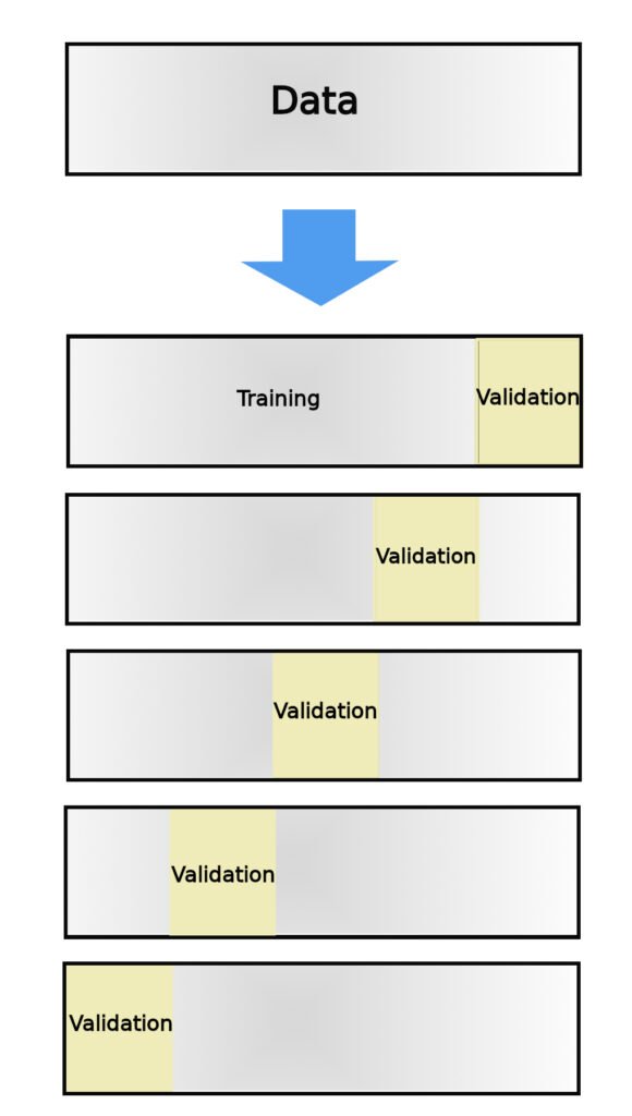
The first critical decision is the choice of a model validation strategy, with N-fold cross-validation often serving as our preferred approach [ref 2]. In this approach, the dataset is divided into N subsets, or folds. The model is trained N times, each time using N-1 folds for training and the remaining fold for validation. Throughout this iterative process, each fold serves as the validation set exactly once, and the final performance metric is typically averaged over these iterations. This technique ensures robust assessment of model performance while mitigating the risk of overfitting.
Another important aspect that demands careful consideration during the stage of model selection is a choice of an appropriate evaluation metric. In the realm of regression problems, where the goal is to predict numeric continuous variables—such as rate coefficient prediction problem in our context —several commonly used metrics come into play, including Mean Absolute Error (MAE), Mean Squared Error (MSE), and Root Mean Squared Error (RMSE) [ref 3]. Each of these metrics bears its unique strengths, with MAE spotlighting the magnitude of absolute errors, MSE placing higher emphasis on larger deviations due to its squared error calculation, and RMSE offering a more interpretable measure by taking the square root of the MSE. Choosing the right evaluation metric is like a compass, helping us make sure our model is accurate and fits well with the specific challenges of our particular regression problem.
Step 6: Selection of a machine learning algorithm
As we reach the concluding phase of our machine learning journey, we encounter a crucial milestone: the selection of the most suitable machine learning algorithm that aligns with the characteristics of our specific problem.
Linear Regression [ref 4], for example, is a suitable choice when the relationship between input features and the target variable appears to be linear. It provides a simple yet effective way to model such relationships.
On the other hand, when we deal with complex, non-linear patterns, as in the case of rate coefficient prediction problem, our preference shifts to more suitable non-linear models like Random Forest [ref 4], XGBoost [ref 5] or Support Vector Regressor [ref 6] as these models can capture complex relationships and patterns within the data that linear models might miss.
However, the process of model selection does not end here. Beyond selecting the right learning algorithm, we need to perform model hyperparameter optimization. Hyperparameters are settings that control the behaviour of the learning algorithm. They include parameters like learning rates, regularisation strengths, and tree depths, among others. Through meticulous fine-tuning of these hyperparameters, we unlock the algorithm’s full potential. This process involves a systematic exploration of diverse hyperparameter combinations, employing techniques like grid search to find the optimal configuration [ref 7].
Finally, in the pursuit of enhancing our model’s predictive performance, we often employ ensemble methods. One such ensemble method that has proven effective in our rate coefficient prediction project is the Voting Regressor. This technique allows us to combine the strengths of multiple individual regression models into a single, more robust predictor. The Voting Regressor operates on the principle of collective wisdom: instead of relying solely on a single regression model, we assemble a diverse ensemble of regression algorithms, each with its unique approach and strengths. These can include Linear Regression, Random Forest, XGBoost, Support Vector Regressor, k-Nearest Neighbours [ref 8] and others.
To wrap things up, machine learning is a powerful tool that, once trained, can provide fast and reasonably accurate predictions. It has proven to be a valuable asset for us and others engaged in solving scientific problems through the application of machine learning methodologies.
A notable and promising aspect of developing machine learning solutions to model systems related to plasma physics lies in the continuous growth of scientific databases including the Quantemol Database (www.quantemolDB.com). This expanding wealth of data presents exciting opportunities not only to enhance the accuracy and effectiveness of our existing machine learning models, but also lays the foundation for the development of even more robust models in our future projects.